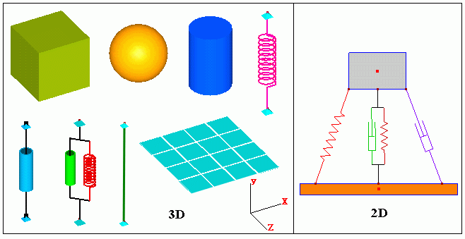
FER/Mech is devoted to 2D and 3D mechanism simulation which include pre/post processor and solver. It allows to design the geometry model, to input the physical parameters to define finite element model, then run the solver and to visualize the analysis results within a very friendly graphical interface.

FER/Mech is developed by using C++ language with the support of OpenGL graphical library on the environment of Microsoft Visual C++ developer studio. With the techniques of object oriented programming and OpenGL programming as well as some new geometrical algorithms, it produces the high image quality and allows to visualize and to operate very easily the computational results.

The main capabilities of FER/Mech include :


Create geometry model 2D and 3D


Define objects properties
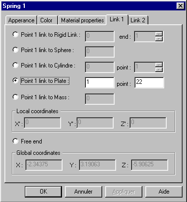

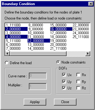
Define boundary conditions

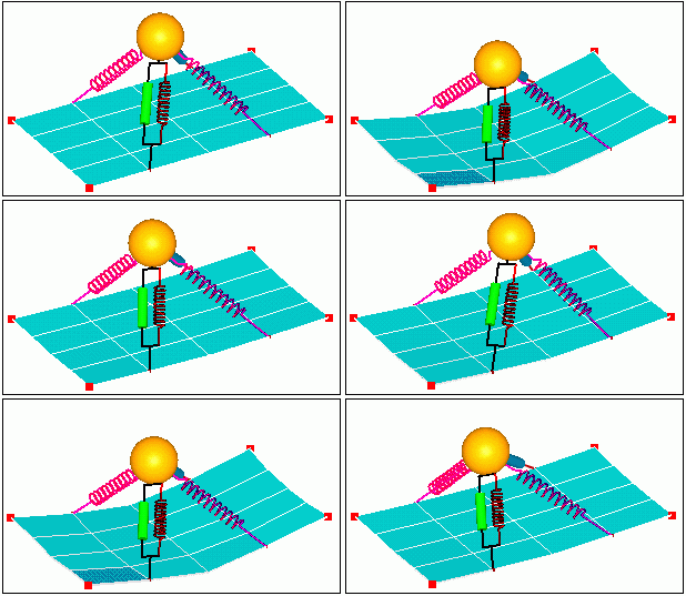
Animation

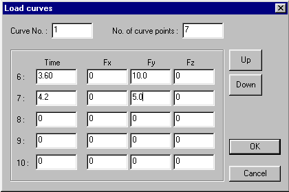
Define load curve

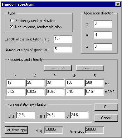
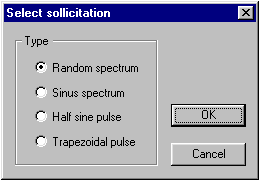
Dynamic loading

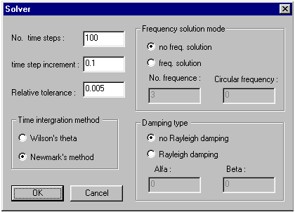
Solver option

XY plot
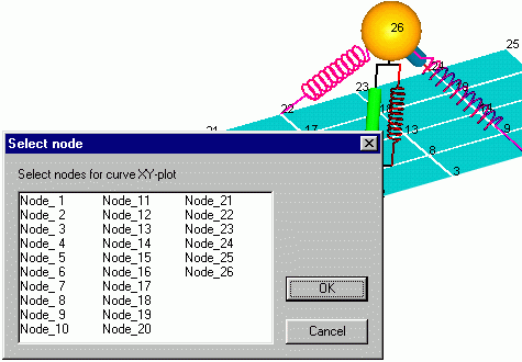
1, Select node
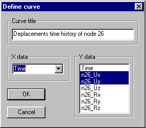
2, Select X, Y data item
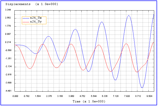
3, Plot curves


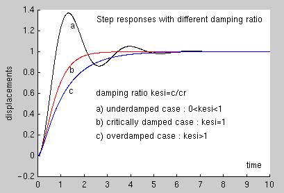
Validation
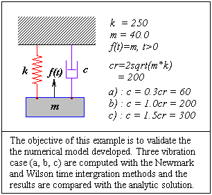


time     Newmark        Wilson           analytic results Matlab program for the analytic solution
a). Results for undamped case (c<cr)
1.00      1.2414465e+00   1.2415120e+00   1.2354857e+00
2.00      1.0573239e+00   1.0573328e+00   1.0603905e+00
3.00      9.0673845e-01   9.0669271e-01   9.0597429e-01
4.00      1.0512690e+00   1.0513037e+00   1.0511105e+00
5.00      9.8559649e-01   9.8558495e-01   9.8587257e-01
6.00      9.9845190e-01   9.9844955e-01   9.9829971e-01
7.00      1.0042779e+00   1.0042834e+00   1.0043202e+00
8.00      9.9740694e-01   9.9740337e-01   9.9741190e-01
9.00      1.0008265e+00   1.0008276e+00   1.0008138e+00
10.0      1.0000110e+00   1.0000111e+00   1.0000185e+00

b). Results for critically damped case (c=cr)
1.00      7.1270785e-01    7.1282989e-01   7.1270250e-01
2.00      9.5957758e-01    9.5959823e-01   9.5957232e-01
3.00      9.9529997e-01    9.9530058e-01   9.9529878e-01
4.00      9.9950079e-01    9.9950043e-01   9.9950060e-01
5.00      9.9994972e-01    9.9994961e-01   9.9994969e-01
6.00      9.9999511e-01    9.9999509e-01   9.9999511e-01
7.00      9.9999954e-01    9.9999953e-01   9.9999954e-01
8.00      9.9999996e-01    9.9999996e-01   9.9999996e-01
9.00      1.0000000e+00    1.0000000e+00   1.0000000e+00
10.0      1.0000000e+00    1.0000000e+00   1.0000000e+00

c). Results for overdamped case (c>cr)
1.00      5.4966400e-01    5.4979719e-01   5.4966130e-01
2.00      8.2659786e-01    8.2664806e-01   8.2659535e-01
3.00      9.3326743e-01    9.3328590e-01   9.3326598e-01
4.00      9.7431850e-01    9.7432528e-01   9.7431776e-01
5.00      9.9011668e-01    9.9011916e-01   9.9011632e-01
6.00      9.9619648e-01    9.9619739e-01   9.9619632e-01
7.00      9.9853625e-01    9.9853658e-01   9.9853617e-01
8.00      9.9943669e-01    9.9943681e-01   9.9943665e-01
9.00      9.9978321e-01    9.9978326e-01   9.9978320e-01
10.0      9.9991657e-01    9.9991659e-01   9.9991657e-01

%compute a step response of spring-mass system 
%by selecting the load f(t) = m, t>0,

k=250;              %spring constant
m=40;               %mass
wn=sqrt(k/m);    %the natural frequency
cr=2*sqrt(m*k)  %the critical damping ratio
t=0:0.01:10;        %computaion time and time step
len = length(t);   %size of time vector t
xt=zeros(1,len);  %creat displacement vector

% a). underdamped case : 0<kesi<1;
c=0.3*cr;
kesi=c/cr;           %damping ratio
wd=sqrt(1-kesi*kesi)*wn; %damped natural frequency
fi=atan((1-kesi*kesi)/kesi);
xt=1-exp(-kesi*wn*t).*sin(wd*t+fi)/sqrt(1-kesi*kesi);
plot(t,xt,'k');
hold on

% b). critically damped case : kesi = 1;
c=1.0*cr;
kesi=c/cr;           %damping ratio
xt=1-exp(-wn*t).*(1+wn*t);
plot(t,xt,'r');

% c). overdamped case : kesi > 1;
c=1.5*cr;
kesi=c/cr;
tt=sqrt(kesi*kesi-1);
xt=1+wn*exp(-kesi*wn*t)/(2*tt).*(exp(-1*tt*wn*t)/...
     ((kesi+tt)*wn)-exp(tt*wn*t)/((kesi-tt)*wn));
plot(t,xt,'b');


Return to principal page